When we talk about markets we often use terms like equilibrium or even market force. We choose this terminology for a reason. The analogy to the well established theories of mechanics and quantum mechanics is intended and the pictures we have in mind are a pendulum or even a simple spring. Their restoring forces seem to model the market forces and therefore we frequently observe argumentations very similar to:
if prices increase, then demand decreases and vice versa finally, because of some process still to be described, the market settles down in an equilibrium (called Walrasian price equilibrium).
As a start, that sounds convincing. There just remains one big question. Is that a good picture? Or, even more to the point:
Are there any justifications for the existence of market forces?
Rather than answering this question (regular readers know my standpoint anyway) I would like to justify why this question is actually reasonable and should be asked and answered. In physics this question is answered to the positive, in economics the situation is a little blurry to say the least. I continue by comparing mechanics with economics in catchwords. Thereby pointing out similarities, but also discrepancies and, in a way, recalling ‘the story so far’.
Basic notions
Let me start with two of the fundamental notions in mechanics, namely position and momentum. In earlier posts we have identified their counterparts in economics as price and demand.
Symmetries
In mechanics the intuition is that momentum is invariant under translation of position. In economics we need demand invariance under price-scaling.
Commutation relations
These symmetries lead to commutation relations of the form ![{[A,B]=\text{id}}](https://s0.wp.com/latex.php?latex=%7B%5BA%2CB%5D%3D%5Ctext%7Bid%7D%7D&bg=ffffff&fg=000000&s=0&c=20201002)
![{[A,B]=A}](https://s0.wp.com/latex.php?latex=%7B%5BA%2CB%5D%3DA%7D&bg=ffffff&fg=000000&s=0&c=20201002)
Bounded representations
Both commutation relations imply that the symmetry groups do not have representations on a finite-dimensional vector space (cf. here).
Unbounded representations
While there are no bounded representations, we get unbounded representations on the Hilbert space 
Uncertainty principle
The uncertainty principle of quantum mechanics is well-known. So far I didn’t write about that here in the blog, but in economics the commutation relations imply inequalities which can also be interpreted as some sort of uncertainty principle. I shall come back to this later.
Time evolution
As described in scientific laws to get the time evolution in quantum mechanics one chooses an action, one uses Legendre transform to obtain the energy, one derives the canonical equations and essentially plugs in the above representation to obtain Schrödingers equation governing the time evolution of a quantum system. That surely sounds more complicated than it actually is.
Why can’t we just do that for markets and obtain market equations governing their time evolution? Now, there are a couple of technical difficulties. The most prominent probably is that the Legendre transform of a market action is not invariant under time translation. Hence, in markets there is no conservation of energy. This fact alone makes the usage of a term like market force a little obscure. What is meant by force if there is no energy or at least no energy conservation?
That essentially is the programme for the rest of the year. I shall spell out the maths behind the uncertainty principle for markets and then delve into the technical details of obtaining a time evolution for markets.
Stay tuned …


 Posted by Uwe Stroinski
  as state space encoding all necessary information on the considered system. The system then is thought to evolve in time on a differentiable
  -dimensional path
  for all
  and
and  . Quite frequently there is a so-called Lagrange function
  on the domain
  and a constraint function
  on the same domain. The path
  is required to minimizes or maximizes the integral
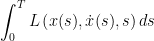
 depending on
  .
. and observe that (under suitable assumptions) this transformation is invertible, i.e. the
  can be expressed as functions of
  and
and  . Next, define the Hamilton operator
![\displaystyle \frac{d x_i}{d t} = - \frac{\partial H}{\partial y_i} \left(=[x_i, H]\right), \frac{d y_i}{d t} = \frac{\partial H}{\partial x_i}\left(=[y_i, H]\right),\frac{d H}{dt} = -\frac{\partial L}{\partial t}](https://s0.wp.com/latex.php?latex=%5Cdisplaystyle+%5Cfrac%7Bd+x_i%7D%7Bd+t%7D+%3D+-+%5Cfrac%7B%5Cpartial+H%7D%7B%5Cpartial+y_i%7D+%5Cleft%28%3D%5Bx_i%2C+H%5D%5Cright%29%2C+%5Cfrac%7Bd+y_i%7D%7Bd+t%7D+%3D+%5Cfrac%7B%5Cpartial+H%7D%7B%5Cpartial+x_i%7D%5Cleft%28%3D%5By_i%2C+H%5D%5Cright%29%2C%5Cfrac%7Bd+H%7D%7Bdt%7D+%3D+-%5Cfrac%7B%5Cpartial+L%7D%7B%5Cpartial+t%7D+&bg=ffffff&fg=000000&s=0&c=20201002)
![{[\cdot,\cdot]}](https://s0.wp.com/latex.php?latex=%7B%5B%5Ccdot%2C%5Ccdot%5D%7D&bg=ffffff&fg=000000&s=0&c=20201002) denotes the commutator bracket
denotes the commutator bracket ![{[a,b]:= ab-ba}](https://s0.wp.com/latex.php?latex=%7B%5Ba%2Cb%5D%3A%3D+ab-ba%7D&bg=ffffff&fg=000000&s=0&c=20201002) . Furthermore, if
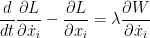
. Furthermore, if  is a constant. That is the aforementioned symmetry.


