As I have told you earlier, my guest is very sceptical about our scientific achievements. What follows are the notes I took, when he gave me a short summary of what he considers ‘our strategy’.
In modern understanding of science, the fundamental laws seem to be consequences of various symmetries of quantities like time, space or similar objects. To make this idea more precise scientists often use mathematical arguments, thereby choosing some set  as state space encoding all necessary information on the considered system. The system then is thought to evolve in time on a differentiable
  -dimensional path
  for all
  and
and  . Quite frequently there is a so-called Lagrange function
  on the domain
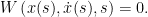
  and a constraint function
  on the same domain. The path
  is required to minimizes or maximizes the integral
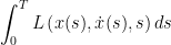
under the constraint
(Under some technical assumptions) a path does exactly that, if it satisfies the Euler-Lagrange equations
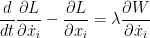
for some function  depending on
  .
.
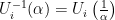
Define  and observe that (under suitable assumptions) this transformation is invertible, i.e. the
  can be expressed as functions of
  and
and  . Next, define the Hamilton operator

as the Legendre transform of . The Legendre transformation is (under some mild technical assumptions) invertible.
Now, (under less mild assumptions, namely holonomic constraints) two things happen. The canonical equations
![\displaystyle \frac{d x_i}{d t} = - \frac{\partial H}{\partial y_i} \left(=[x_i, H]\right), \frac{d y_i}{d t} = \frac{\partial H}{\partial x_i}\left(=[y_i, H]\right),\frac{d H}{dt} = -\frac{\partial L}{\partial t}](https://s0.wp.com/latex.php?latex=%5Cdisplaystyle+%5Cfrac%7Bd+x_i%7D%7Bd+t%7D+%3D+-+%5Cfrac%7B%5Cpartial+H%7D%7B%5Cpartial+y_i%7D+%5Cleft%28%3D%5Bx_i%2C+H%5D%5Cright%29%2C+%5Cfrac%7Bd+y_i%7D%7Bd+t%7D+%3D+%5Cfrac%7B%5Cpartial+H%7D%7B%5Cpartial+x_i%7D%5Cleft%28%3D%5By_i%2C+H%5D%5Cright%29%2C%5Cfrac%7Bd+H%7D%7Bdt%7D+%3D+-%5Cfrac%7B%5Cpartial+L%7D%7B%5Cpartial+t%7D+&bg=ffffff&fg=000000&s=0&c=20201002)
are equivalent to the Euler Lagrange equations. Here ![{[\cdot,\cdot]}](https://s0.wp.com/latex.php?latex=%7B%5B%5Ccdot%2C%5Ccdot%5D%7D&bg=ffffff&fg=000000&s=0&c=20201002) denotes the commutator bracket
denotes the commutator bracket ![{[a,b]:= ab-ba}](https://s0.wp.com/latex.php?latex=%7B%5Ba%2Cb%5D%3A%3D+ab-ba%7D&bg=ffffff&fg=000000&s=0&c=20201002) . Furthermore, if does not explicitly depend on time, then
. Furthermore, if does not explicitly depend on time, then  is a constant. That is the aforementioned symmetry. , the energy, is invariant under time translations.
Given all that, the solution of the minimisation or maximisation problem can then be given (either in the Heisenberg picture) as

or (in the in this case equivalent Schrödinger picture,) as an equation on the state space

This description is equivalent (under mild technical assumptions) to the following initial value problem:

where the operator is the ‘law’. More technically, the law is the generator of a strongly continuous (semi-)group of (in this case linear and unitary) operators acting on (the Hilbert space) . As an example of this process he mentioned the Schrödinger equation governing quantum mechanical processes.
His conclusion was that the frequently appearing ‘technical assumptions’ in the above derivation make it highly unlikely for laws to exist even for systems with, what he calls, no emergent properties. ‘If that was true’, I thought ‘then … bye bye theory of everything!’ He explained further, that under no reasonable circumstances it is possible to extrapolate these laws to the emergent situation. I am not sure, whether I understand completely what he means by that, but his summary on how we find scientific laws is in my opinion way too simple. It can’t be true and I told him.
With just a couple of ink strokes he derived the commutation relations for exchange markets from microeconomic theory. That left me speechless, since I always thought, that there cannot be ‘market laws’. Markets are on principle unpredictable! They are, or?


![\displaystyle [p_i,d_j]=i \mu_i p_i \delta_{i,j} \ \ \ \ \ (1)](https://s0.wp.com/latex.php?latex=%5Cdisplaystyle++%09%09+%09%09%5Bp_i%2Cd_j%5D%3Di+%5Cmu_i+p_i+%5Cdelta_%7Bi%2Cj%7D+%5C+%5C+%5C+%5C+%5C+%281%29&bg=ffffff&fg=000000&s=0&c=20201002)


![{ab = \frac{1}{2}[a,b]_+ + \frac{1}{2i}i[a,b]}](https://s0.wp.com/latex.php?latex=%7Bab+%3D+%5Cfrac%7B1%7D%7B2%7D%5Ba%2Cb%5D_%2B+%2B+%5Cfrac%7B1%7D%7B2i%7Di%5Ba%2Cb%5D%7D&bg=ffffff&fg=000000&s=0&c=20201002)
![{[a,b]_+=ab+ba}](https://s0.wp.com/latex.php?latex=%7B%5Ba%2Cb%5D_%2B%3Dab%2Bba%7D&bg=ffffff&fg=000000&s=0&c=20201002)
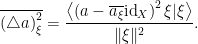
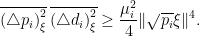
![\displaystyle \begin{array}{rcl} \overline{\left(\triangle p_i \right)^2_\xi} \, \overline{\left(\triangle d_i \right)^2_\xi} & \geq & \left\langle\frac{1}{2} [d_i - \overline{d_i} \text{id}_X, p_i - \overline{p_i} \text{id}_X]_+\xi|\xi\right\rangle^2 \\ & & \qquad +\left\langle\frac{1}{2i} [d_i - \overline{d_i} \text{id}_X, p_i - \overline{p_i} \text{id}_X]\xi|\xi\right\rangle^2 \end{array}](https://s0.wp.com/latex.php?latex=%5Cdisplaystyle+%5Cbegin%7Barray%7D%7Brcl%7D+%5Coverline%7B%5Cleft%28%5Ctriangle+p_i+%5Cright%29%5E2_%5Cxi%7D+%5C%2C+%5Coverline%7B%5Cleft%28%5Ctriangle+d_i+%5Cright%29%5E2_%5Cxi%7D+%26+%5Cgeq+%26+%5Cleft%5Clangle%5Cfrac%7B1%7D%7B2%7D+%5Bd_i+-+%5Coverline%7Bd_i%7D+%5Ctext%7Bid%7D_X%2C+p_i+-+%5Coverline%7Bp_i%7D+%5Ctext%7Bid%7D_X%5D_%2B%5Cxi%7C%5Cxi%5Cright%5Crangle%5E2+%5C%5C+%26+%26+%5Cqquad+%2B%5Cleft%5Clangle%5Cfrac%7B1%7D%7B2i%7D+%5Bd_i+-+%5Coverline%7Bd_i%7D+%5Ctext%7Bid%7D_X%2C+p_i+-+%5Coverline%7Bp_i%7D+%5Ctext%7Bid%7D_X%5D%5Cxi%7C%5Cxi%5Cright%5Crangle%5E2+%5Cend%7Barray%7D+&bg=ffffff&fg=000000&s=0&c=20201002)
![\displaystyle \begin{array}{rcl} \overline{\left(\triangle p_i \right)^2_\xi} \, \overline{\left(\triangle d_i \right)^2_\xi} & \geq & \left\langle\frac{1}{2i} [d_i - \overline{d_i} \text{id}_X, p_i - \overline{p_i} \text{id}_X]\xi|\xi\right\rangle^2 \\ & \geq & \left\langle\frac{1}{2i} [d_i,p_i]\xi|\xi\right\rangle^2. \end{array}](https://s0.wp.com/latex.php?latex=%5Cdisplaystyle+%5Cbegin%7Barray%7D%7Brcl%7D+%5Coverline%7B%5Cleft%28%5Ctriangle+p_i+%5Cright%29%5E2_%5Cxi%7D+%5C%2C+%5Coverline%7B%5Cleft%28%5Ctriangle+d_i+%5Cright%29%5E2_%5Cxi%7D+%26+%5Cgeq+%26+%5Cleft%5Clangle%5Cfrac%7B1%7D%7B2i%7D+%5Bd_i+-+%5Coverline%7Bd_i%7D+%5Ctext%7Bid%7D_X%2C+p_i+-+%5Coverline%7Bp_i%7D+%5Ctext%7Bid%7D_X%5D%5Cxi%7C%5Cxi%5Cright%5Crangle%5E2+%5C%5C+%26+%5Cgeq+%26+%5Cleft%5Clangle%5Cfrac%7B1%7D%7B2i%7D+%5Bd_i%2Cp_i%5D%5Cxi%7C%5Cxi%5Cright%5Crangle%5E2.+%5Cend%7Barray%7D+&bg=ffffff&fg=000000&s=0&c=20201002)


 Posted by Uwe Stroinski
  on an appropriate Hilbert space.
 . This, in a way, is the simplest non-finite dimensional Hilbert space and therefore an unsurprising first choice. Thus, the state of the market with
  goods is described by a function
  , then the demand
  is given as a differential operator

 has the same domain as
  as
as  . Then, the price operator
  is given as a multiplication operator

 are self-adjoint,
 ![\displaystyle \left[p_i,z_i\right]\xi = \left[p_i,d_i\right]\xi = -i \mu_i \left(e_i \cdot \frac{d}{d x_i}\xi - e_i \cdot \xi - e_i \cdot \frac{d}{d x_i} \xi\right)= i \mu_i p_i \xi](https://s0.wp.com/latex.php?latex=%5Cdisplaystyle+%5Cleft%5Bp_i%2Cz_i%5Cright%5D%5Cxi+%3D+%5Cleft%5Bp_i%2Cd_i%5Cright%5D%5Cxi+%3D+-i+%5Cmu_i+%5Cleft%28e_i+%5Ccdot+%5Cfrac%7Bd%7D%7Bd+x_i%7D%5Cxi+-+e_i+%5Ccdot+%5Cxi+-+e_i+%5Ccdot+%5Cfrac%7Bd%7D%7Bd+x_i%7D+%5Cxi%5Cright%29%3D+i+%5Cmu_i+p_i+%5Cxi+&bg=ffffff&fg=000000&s=0&c=20201002)
 of and demands
  for goods, by observables acting on some Hilbert space
  .
. of good
  for all goods
 ![\displaystyle \left[p_i, d_j\right]=i \mu_i p_i \delta_{i,j}](https://s0.wp.com/latex.php?latex=%5Cdisplaystyle++%09%09%09%5Cleft%5Bp_i%2C+d_j%5Cright%5D%3Di+%5Cmu_i+p_i+%5Cdelta_%7Bi%2Cj%7D+%09%09&bg=ffffff&fg=000000&s=0&c=20201002)
 satisfy a commutation relation
 ![{[A,B]=\textnormal{id}_X}](https://s0.wp.com/latex.php?latex=%7B%5BA%2CB%5D%3D%5Ctextnormal%7Bid%7D_X%7D&bg=ffffff&fg=000000&s=0&c=20201002) , then not both can be bounded simultaneously. Since there are no unbounded linear operators on finite dimensional vector spaces, the Hilbert space then must be infinite dimensional.
, then not both can be bounded simultaneously. Since there are no unbounded linear operators on finite dimensional vector spaces, the Hilbert space then must be infinite dimensional. we observe that our commutation relation is
 ![{[A,B]=A}](https://s0.wp.com/latex.php?latex=%7B%5BA%2CB%5D%3DA%7D&bg=ffffff&fg=000000&s=0&c=20201002) which is certainly different from the quantum situation.
which is certainly different from the quantum situation. for all
  . Assume furthermore
 ![{[A,B]= A}](https://s0.wp.com/latex.php?latex=%7B%5BA%2CB%5D%3D+A%7D&bg=ffffff&fg=000000&s=0&c=20201002) and as induction hypothesis
and as induction hypothesis ![{[A^n,B]= nA^n}](https://s0.wp.com/latex.php?latex=%7B%5BA%5En%2CB%5D%3D+nA%5En%7D&bg=ffffff&fg=000000&s=0&c=20201002) . Then
. Then ![{[A^{n+1},B]= A[A^n,B]+[A,B]A^n=nA^{n+1}+A^{n+1}=(n+1)A^{n+1}}](https://s0.wp.com/latex.php?latex=%7B%5BA%5E%7Bn%2B1%7D%2CB%5D%3D+A%5BA%5En%2CB%5D%2B%5BA%2CB%5DA%5En%3DnA%5E%7Bn%2B1%7D%2BA%5E%7Bn%2B1%7D%3D%28n%2B1%29A%5E%7Bn%2B1%7D%7D&bg=ffffff&fg=000000&s=0&c=20201002) . The norm estimate
. The norm estimate ![{n \|A^n\| = \|[A^n,B]\|\leq 2 \|A^n\| \|B\|}](https://s0.wp.com/latex.php?latex=%7Bn+%5C%7CA%5En%5C%7C+%3D+%5C%7C%5BA%5En%2CB%5D%5C%7C%5Cleq+2+%5C%7CA%5En%5C%7C+%5C%7CB%5C%7C%7D&bg=ffffff&fg=000000&s=0&c=20201002) yields a contradiction since
yields a contradiction since  and
and  is unbounded and/or the commutation relation
  for
for  . This goods are being traded and therefore we need to talk about prices and demand. Call
  . What else do we need?
 . The day after, no increase of demand for fridges, cars, credits aso. was observed. That was no surprise for economists. Where should a change of demand come from? A redefinition of the currency is not enough to generate demand. That is generally believed and a pillar in the following argumentation.
 and then scale by a factor
  we obtain a scaling by the factor
  . Scaling with 1 is the neutral element and for each scale factor
  .
. . Of course, in the moment you can think of
  or
or  . On the other hand, it is always good to be suspicious and fixing the dimension to be finite might be premature. Observables are self-adjoint operators on this Hilbert space and satisfy the following axioms:
 for all
  in the domain
  of
of  be a strongly continuous family of unitary operators on
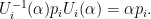
 satisfies the following properties for all
  and
and  :
:

 and observe


 to be a strongly continuous group of unitary operators acting on
  . Set
. Set  and with
  it follows that
 yields
![\displaystyle \left[p_i, A_i\right] = p_i. \ \ \ \ \ (1)](https://s0.wp.com/latex.php?latex=%5Cdisplaystyle++%09+%09%5Cleft%5Bp_i%2C+A_i%5Cright%5D+%3D+p_i.+%5C+%5C+%5C+%5C+%5C+%281%29&bg=ffffff&fg=000000&s=0&c=20201002)
 also commutes with
  for any
  . Hence
  and
and  for some
  . Furthermore, since scaling of one price does not influence scaling of the others (i.e.,
 ![{\left[p_i, U_j(\alpha)\right]=0}](https://s0.wp.com/latex.php?latex=%7B%5Cleft%5Bp_i%2C+U_j%28%5Calpha%29%5Cright%5D%3D0%7D&bg=ffffff&fg=000000&s=0&c=20201002) for
for  ) we can use (
![\displaystyle \left[p_i, i \mu_i A_j - \omega_i \textnormal{id}_X\right] = i \mu_i p_i \delta_{i,j}.](https://s0.wp.com/latex.php?latex=%5Cdisplaystyle++%09%5Cleft%5Bp_i%2C+i+%5Cmu_i+A_j+-+%5Comega_i+%5Ctextnormal%7Bid%7D_X%5Cright%5D+%3D+i+%5Cmu_i+p_i+%5Cdelta_%7Bi%2Cj%7D.+&bg=ffffff&fg=000000&s=0&c=20201002)
 is an observable and is invariant under price-scaling. Economic intuition therefore leads us to identify this operator with the demand respectively excess demand for good
  . The real parameter